Introduction
Although data science projects often employ large amounts of numeric data, some projects examine patterns within text and require a different set of tools. In this code-through tutorial, we are going to explore several packages in R that enable researchers to analyze qualitative data sets and discovercool patterns. We are also going to create two word clouds based on movie plot summaries.
In order to complete this tutorial, you will need access to R or RStudio. If you are not familiar with either of these software or would like a refresher on the basics, check out the first steps of my previous code-through here. I walk you through the entire set-up process beginning with the software.
If you’re all set to go with R and RStudio, then proceed below:
Set-Up
Library of Packages
Before we begin analyzing and our data and creating word clouds, first, we need to load a few packages into our ‘library’. Specifically we need the following packages:
library( dplyr ) # helps organize our data
library(kableExtra) # creates elegant tables for output
library( quanteda ) # processes our textual data for anaylsis
library( wordcloud2 ) # creates the wordclouds
You can easily install all of these packages with the following code:
install.packages("nameofpackage")
Data
Now that we have our packages installed, the next thing that we need is our dataset. For the purposes of this code-through we are going to be using a dataset of over 5000 movies from IMDB that we will access from data.world: https://data.world/studentoflife/imdb-top-250-lists-and-5000-or-so-data-records
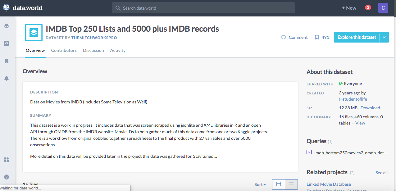
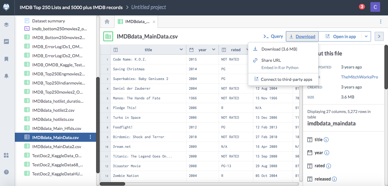
We will click the blue Explore this dataset button and then scroll down to select the IMDBdata_MainData.csv dataset.
Next, we will click the download button where we will select the download URL for R.
Data.World provides us with the exact code we need to get started and import our data. Therefore we will copy and paste into a codeblock as follows:
df <- read.csv("https://query.data.world/s/rr46ndg7fyne54q7oonmvzxbaxg3zn", header=TRUE, stringsAsFactors=FALSE);
Preview Dataset
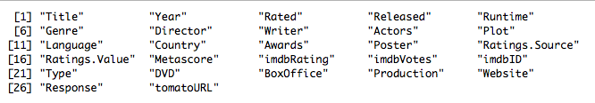
A quick peek at the column names of the dataset reveal the various fields available for us to use to explore the 5,000+ movies in the set.
colnames(df)
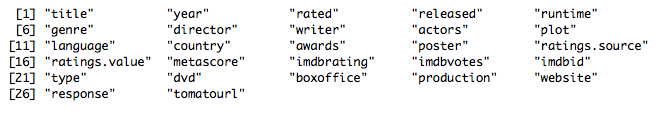
For ease of reference, we will change all of these titles to be lowercase with the following function:
colnames(df)<- tolower(colnames(df))
colnames(df)
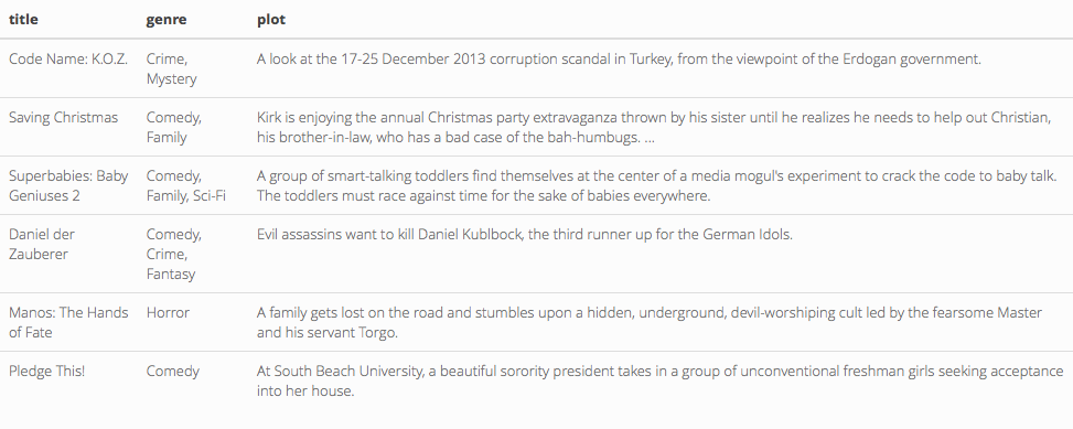
For our analysis, we will focus specifically on the movie titles, genres, and plots, so we will create a smaller dataset with only these variables:
dat <- df[c("title", "genre", "plot" )]
A preview of this dataset gives us a glimpse into what we’re working with:
head( dat ) %>% kable() %>% kable_styling()
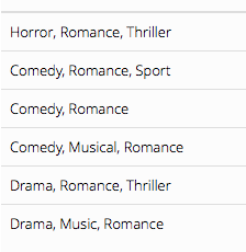
Now we will create an even smaller dataset of only romance movies using the grep() function which allows us to search through text for specfic key words. Here, we will search for all movies that have romance listed as either its only genre or at least one of its genres:
grep( pattern="romance", x=dat$genre, value=TRUE, ignore.case=TRUE ) %>% head() %>% kable() %>% kable_styling()
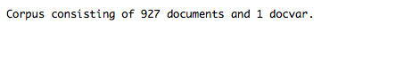
Using the grepl() function we will find all 927 movies that belong to the romance genre:
romance <- grepl( "romance", dat$genre, ignore.case = T )
sum(romance)
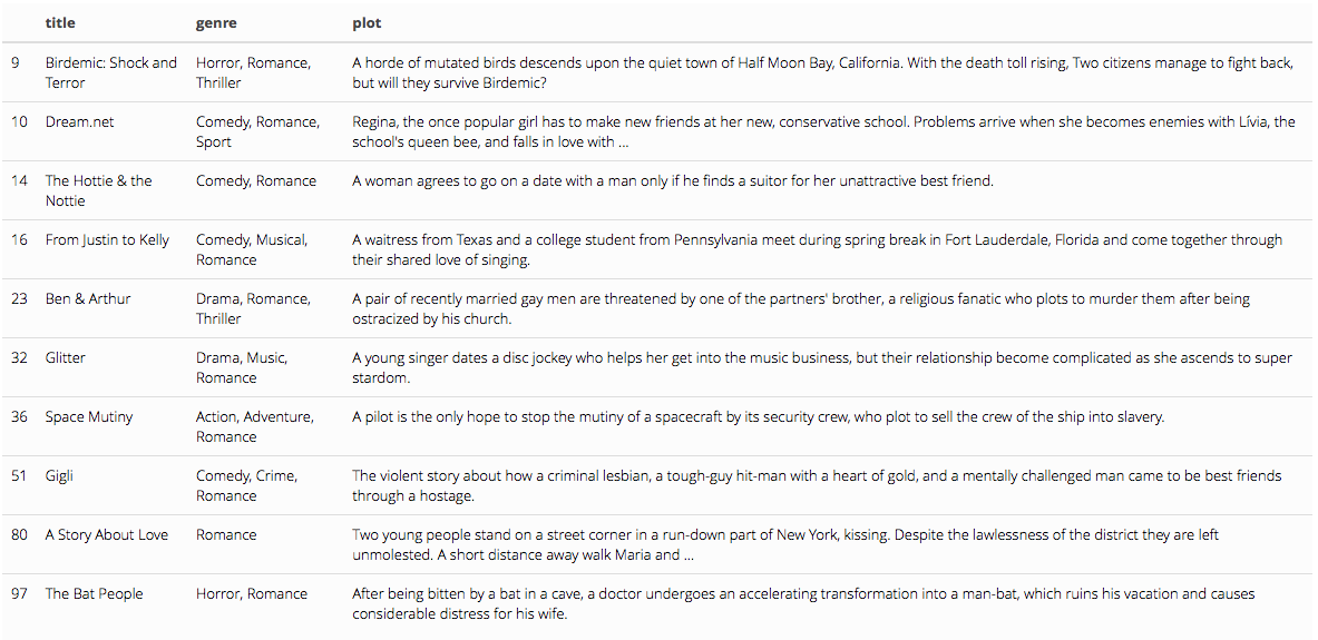
We will use this criteria to segment out the romance movies:
dat.romance <- dat[ romance, c("title", "genre", "plot") ]
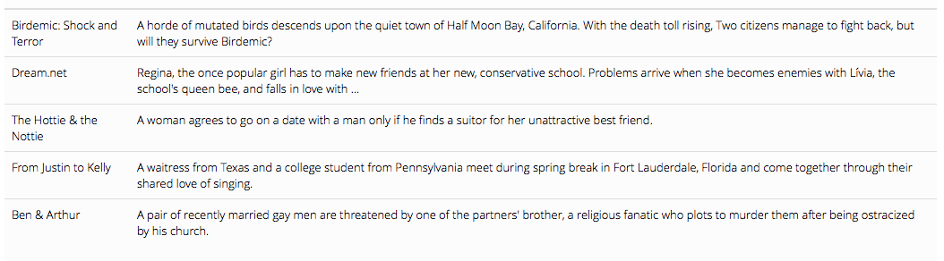
dat.romance %>% head(10) %>% kable() %>% kable_styling()
Now that we have a collection of romance movie titles, we will focus on examining the plots of the movies to see if there are any similarities or common keywords across the summaries:
corp.romance <- corpus( dat.romance, docid_field="title", text_field="plot" )
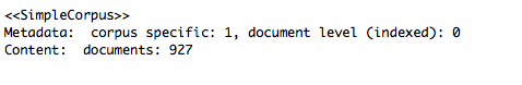
corp.romance
#
corp.romance[1:5] %>% kable() %>% kable_styling()
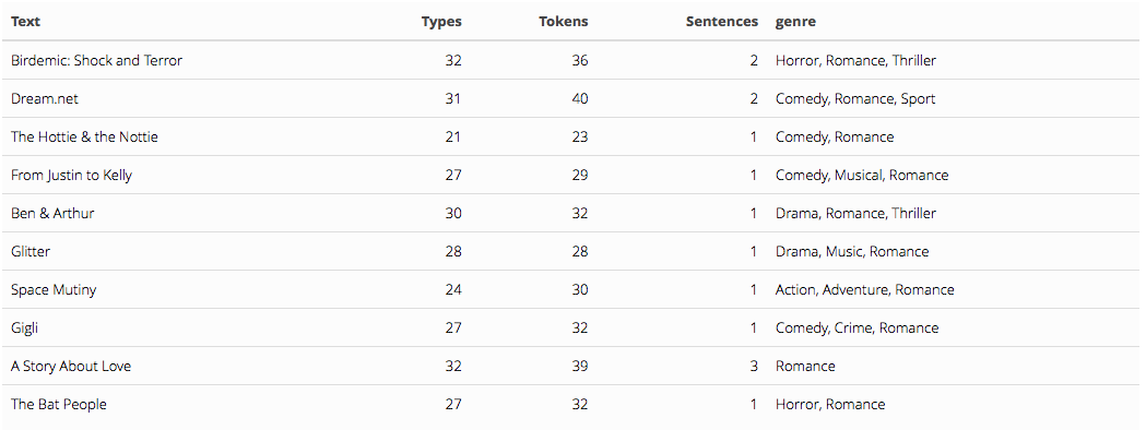
# summarize corpus
summary(corp.romance)[1:10,] %>% kable() %>% kable_styling()
# Process text
# remove mission statements that are less than 1 sentence long
corp.romance <- corpus_trim( corp.romance, what="sentences", min_ntoken=1 )
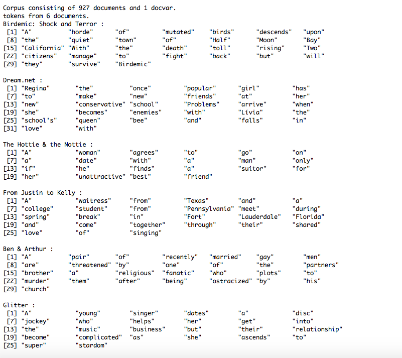
corp.romance
# remove punctuation
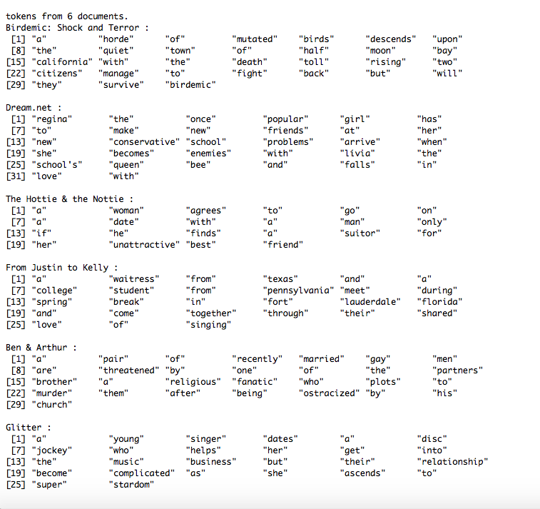
tokens.romance <- tokens( corp.romance, what="word", remove_punct=TRUE )
head( tokens.romance )
# convert to lower case
tokens.romance <- tokens_tolower( tokens.romance, keep_acronyms=TRUE )
head( tokens.romance )
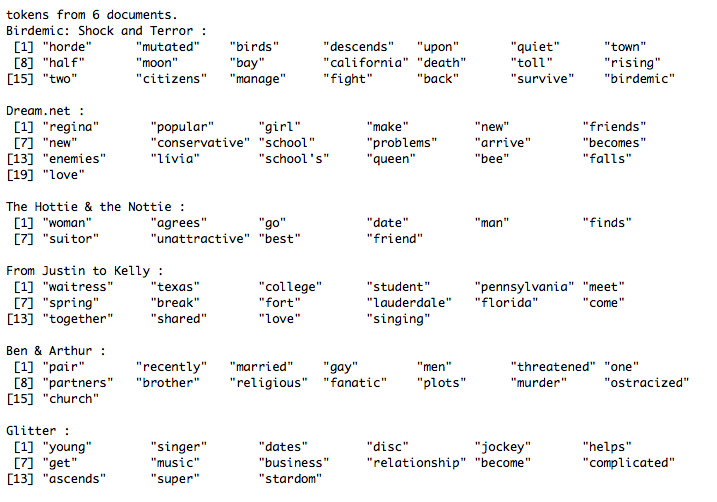
In order to make the data set more precise, we will remove all of the articles from the data set:
tokens.romance <- tokens_remove( tokens.romance, c( stopwords("english"), "nbsp" ), padding=F )
head(tokens.romance)
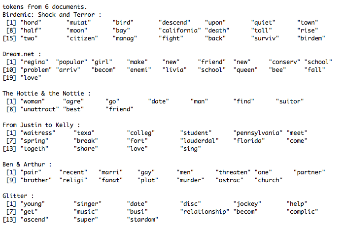
In order to consolidate similar words, we will stem the data set:
# stem the words in the token list:
tokens.romance <- tokens_wordstem( tokens.romance )
head( tokens.romance )
We can see which words commonly occur together:
# find frequently co-occuring words (typically compound words)
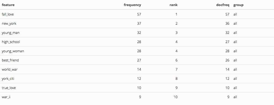
ngram.romance <- tokens_ngrams( tokens.romance, n=2 ) %>% dfm()
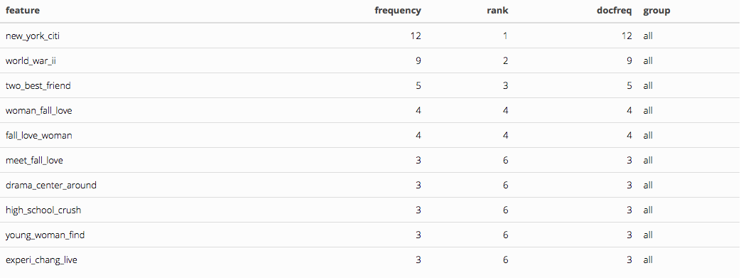
ngram.romance %>% textstat_frequency( n=10 ) %>% kable() %>% kable_styling()
ngram.romance3 <- tokens_ngrams( tokens.romance, n=3 ) %>% dfm()
ngram.romance3 %>% textstat_frequency( n=10 ) %>% kable() %>% kable_styling()
Finally we can see which words are most common in the romance movie plot summaries:
tokens.romance %>% dfm( stem=T ) %>% topfeatures( ) %>% kable() %>% kable_styling()
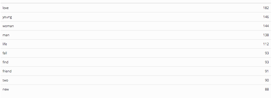
Unsurprisingly(!!) love is the number one most frequently used word followed by young, woman, and man.
Word Clouds
Now that we’ve previewed our data step-by-step, we can create a wordcloud. We will repeat some of our previous steps in a more automated format using the tm() package. If you do not have it installed, once again you can install it via install.packages("tm")
library( tm ) # package for processing text
Romance Movies
For our first word cloud, we will create a new dataset creating only our plots from romance movies:
#Create a vector containing only the text
romance.plot <- dat.romance$plot
Then we will create a new Corpus consisting solely of the plot:
# Create a corpus
romance.docs <- Corpus(VectorSource(romance.plot))
romance.docs
Afterwords, we will go through the same steps that we did above to clean our data set:
romance.docs <- romance.docs %>%
  tm_map(removeNumbers) %>%
  tm_map(removePunctuation) %>%
  tm_map(stripWhitespace)
romance.docs <- tm_map(romance.docs, content_transformer(tolower))
romance.docs <- tm_map(romance.docs, removeWords, stopwords("english"))
And once again find our most frequently used words:
romance.dtm <- TermDocumentMatrix(romance.docs)
romance.matrix <- as.matrix(romance.dtm)
romance.words <- sort(rowSums(romance.matrix),decreasing=TRUE)
romance.df <- data.frame(word = names(romance.words),freq=romance.words)
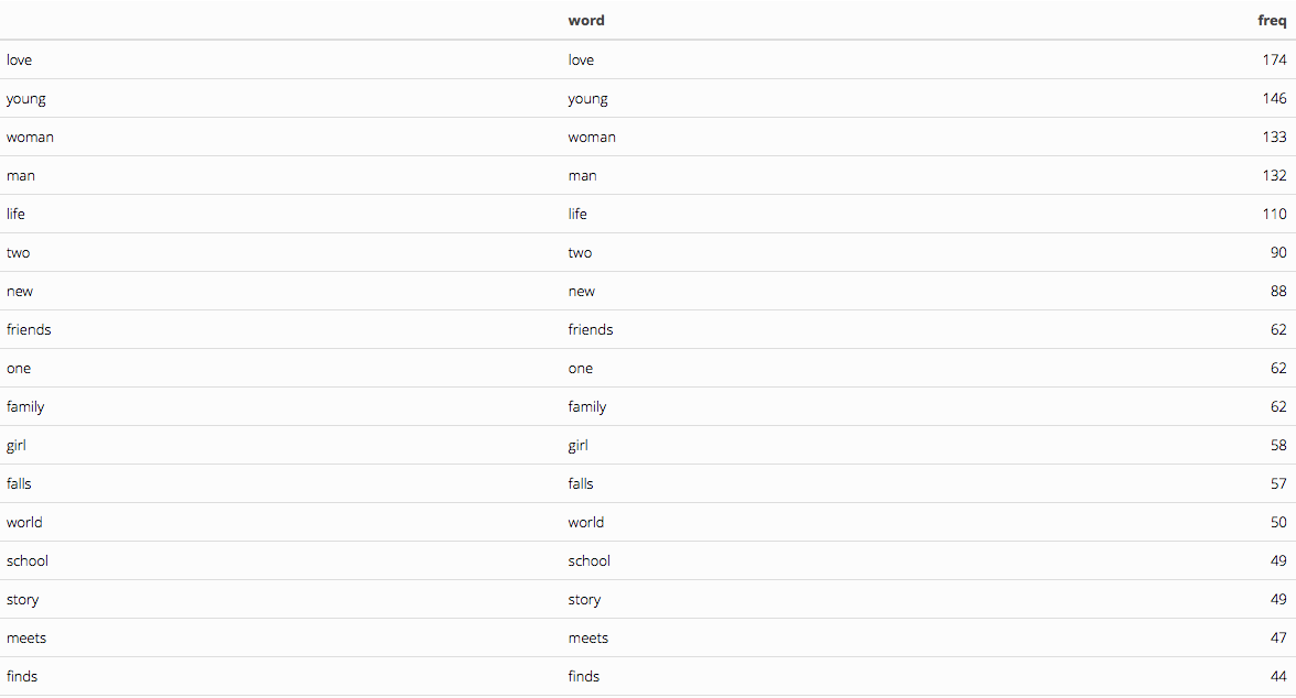
romance.df %>% kable() %>% kable_styling()
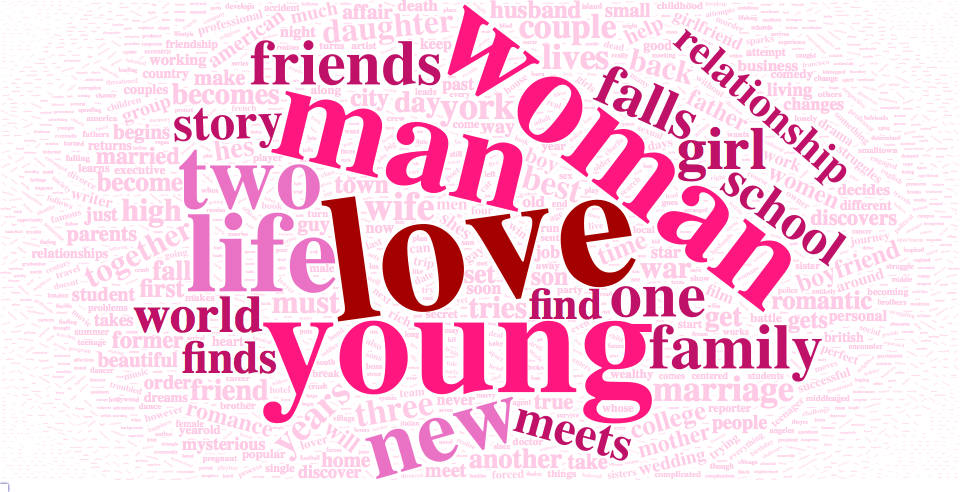
Finally, we will create a color pallete and voila! we’ve created a word cloud based on over 900 romance movie plots:
pallete <- mutate(romance.df, color = cut(freq, breaks = c(0, 40, 80, 120, 160, Inf),
             labels = c("#FFCAE5", "#BF1168","#EA72C4", "#FF167F", "A40000"),
             include.lowest = TRUE))

romance.word.cloud <- wordcloud2(data = pallete, color = pallete$color)
romance.word.cloud
If we would like to save our widget, then we can save it as an html, png, and pdf file.
# save it in html
library("htmlwidgets")
library(webshot)

saveWidget(romance.word.cloud,"romancewordcloud.html",selfcontained = F)

# and in png or pdf
webshot("romancewordcloud.html","romancewordcloud.png", delay =60, vwidth = 960, vheight=480)
Crime Movies
Finally, for a comparison word cloud, we will create a second data set for crime movies to find out how keywords for this genre differ from romance movies:
grep( pattern="crime", x=dat$genre, value=TRUE, ignore.case=TRUE ) %>% head() %>% kable() %>% kable_styling()
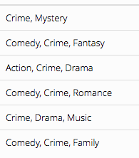
We find that there are 930 movies with crime listed as a genre:
crime <- grepl( "crime", dat$genre, ignore.case = T )
sum(crime)
Once again, we will use this criteria to segment out the crime movies:
dat.crime <- dat[ crime, c("title", "genre", "plot") ]
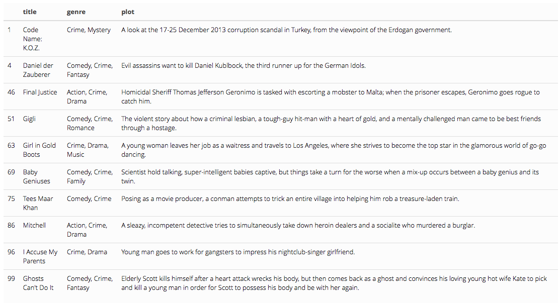
dat.crime %>% head(10) %>% kable() %>% kable_styling()
Now we extract the crime plots:
#Create a vector containing only the text
crime.plot <- dat.crime$plot
Create a crime corpus:
# Create a corpus
crime.docs <- Corpus(VectorSource(crime.plot))
crime.docs

crime.docs <- crime.docs %>%
  tm_map(removeNumbers) %>%
  tm_map(removePunctuation) %>%
  tm_map(stripWhitespace)
crime.docs <- tm_map(crime.docs, content_transformer(tolower))
crime.docs <- tm_map(crime.docs, removeWords, stopwords("english"))
crime.dtm <- TermDocumentMatrix(crime.docs)
crime.matrix <- as.matrix(crime.dtm)
crime.words <- sort(rowSums(crime.matrix),decreasing=TRUE)
crime.df <- data.frame(word = names(crime.words),freq=crime.words)
crime.df %>% kable() %>% kable_styling()
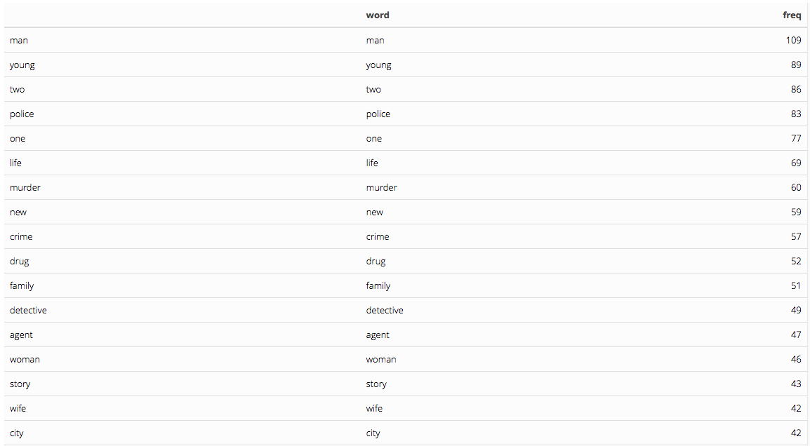
For crime moves, we find that our most frequent word is man and young comes in second place again. The third most frequently used word here is ‘two’, but police is not far behind for fourth place, as would be expected in a crime movie.
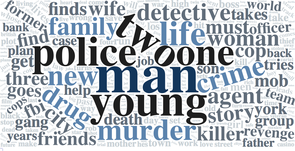
Now we create a new color pallete and just like that we have a second word cloud based on over 900 crime movie plots:
crime.pallete <- mutate(crime.df, color = cut(freq, breaks = c(0, 25, 50, 75, 100, Inf),
             labels = c("#C9D1D6", "#616D7A","#5B83AD", "#1E1E1E", "#13365B"),
             include.lowest = TRUE))

crime.word.cloud <- wordcloud2(data = crime.pallete, color = crime.pallete$color)
crime.word.cloud
# save it in html
library("htmlwidgets")
library(webshot)

saveWidget(crime.word.cloud,"crimewordcloud.html",selfcontained = F)

# and in png or pdf
webshot("crimewordcloud.html","crimewordcloud.png", delay =60, vwidth = 960, vheight=480)
Comparison and Conclusion:
Now that we have completed this tutorial, we have been able to discover some similarities in individual words between the two word clouds:
However, the collective data from both sets of plots clearly displays how some of the same keywords can carry very different meanings between genres. We have also learned two methods for processing data: the first method using grep(), grepl() and quanteda() is quite a bit longer than using the tm() methods, but it has its perks of letting us see our data at every stage. Similarly tm() does not provide as much insight into into textual analysis, but for the purposes of quick projects like the wordclouds, it makes the process much easier!
Resources
Now that you have created your first wordcloud, I encourage you to try out the features and give it a try yourself! The following links contain tutorials and resources to guide you each step of the way:
Create a word cloud with r This tutorial from ‘towards data science’ by Celine Van den Rul served as the inspiration for this code-through and includes great step-by-step details on all of the features of wordcloud2() as well as its more basic predecessor wordcloud(). Both packages have unique benefits!
Wordcloud
This article focuses on the first wordcloud() and has lots of great insight.
R Graph Gallery: Wordcloud2 The R Graph Gallery has excellent tutorials on various data visualization strategies in R and is a wonderful guide for Wordcloud2.
CRAN also has wonderful resources for wordcloud2() available for view here in PDF form and here in website form.
Webshot is a neat package that allows us to create static saved images of the ever-changing word clouds that we create.
Coolors is a great site to find colors for your word cloud palettes.
Last, but certainly not least, Data.World is an excellent place to find data on just about any subject and the pre-configured R URL download links are especially helpful!
About The Author
This code-through tutorial was created by Courtney Stowers for CPP 527 Data Science 2 in the Master of Science in Program Evaluation and Data Analytics program at Arizona State University. She can be contacted at: courtney.stowers@asu.edu.
Clip art credit: Wokandapix, Pixabay